number of breaks, should be one more than the number of colors given
breaks
actual breaks used to assign colors to values; if missing, the function subsamples values and uses equally sized intervals between min and max or zlim[0] and zlim[1] if defined
col
color definition, can be a character vector with nbreaks - 1 elements or a function such as heat.colors
key.pos
position for the legend, 1 (bottom), 2 (left), 3 (top), or 4 (right). If NULL (the default), do not plot a legend.
bands
integer vector with band numbers to plot (this must be band numbers, not band names)
t
integer vector with time indexes to plot (this must be time indexes, not date / time)
rgb
bands used to assign RGB color channels, vector of length 3 (this must be band numbers, not band names)
zlim
vector of length 2, defining the minimum and maximum values to either derive breaks, or define black and white values in RGB plots
gamma
gamma correction value, used for RGB plots only
periods.in.title
logical value, if TRUE, the title of plots includes the datetime period length as ISO 8601 string
join.timeseries
logical, for pure time-series plots, shall time series of multiple bands be plotted in a single plot (with different colors)?
axes
logical, if TRUE, plots include axes
ncol
number of columns for arranging plots with layout(), see Details
nrow
number of rows for arranging plots with layout(), see Details
downsample
length-one integer or logical value used to select only every i-th pixel (in space only) for faster plots; by default (TRUE), downsampling will be determined automatically based on the resolution of the graphics device; set to FALSE to avoid downsampling.
na.color
color used to plot NA pixels
Details
The style of the plot depends on provided parameters and on the shape of the cube, i.e., whether it is a pure time series and whether it contains multiple bands or not. Multi-band, multi-temporal images will be arranged with layout() such that bands are represented by columns and time is represented by rows. Time series plots can be combined to a single plot by setting join.timeseries = TRUE. The layout can be controlled with ncol and nrow, which define the number of rows and columns in the plot layout. Typically, only one of ncol and nrow is provided. For multi-band, multi-temporal plots, the actual number of rows or columns can be less if the input cube has less bands or time slices.
The downsample argument is used to speed-up plotting if the cube has much more pixels than the graphics device. If set to a scalar integer value > 1, the value is used to skip pixels in the spatial dimensions. For example, setting downsample = 4 means that every fourth pixel is used in the spatial dimensions. If TRUE (the default) downsample is derived automatically based on the sizes of the cube and the graphics device. If 1 or FALSE, no additional downsampling is performed. Notice that downsampling is only used for plotting. The size of the data cube (and hence the computation time to process the data cube) is not modified.
Note
If caching is enabled for the package (see gdalcubes_options), repeated calls of plot for the same data cube will not reevaluate the cube. Instead, the temporary result file will be reused, if possible.
Some parts of the function have been copied from the stars package (c) Edzer Pebesma
Examples
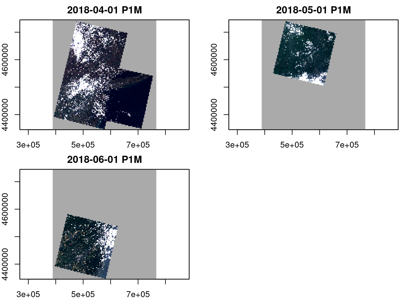
# create image collection from example Landsat data only # if not already done in other examplesif (!file.exists(file.path(tempdir(), "L8.db"))) { L8_files <-list.files(system.file("L8NY18", package ="gdalcubes"),".TIF", recursive =TRUE, full.names =TRUE)create_image_collection(L8_files, "L8_L1TP", file.path(tempdir(), "L8.db"), quiet =TRUE) }L8.col =image_collection(file.path(tempdir(), "L8.db"))v =cube_view(extent=list(left=388941.2, right=766552.4, bottom=4345299, top=4744931, t0="2018-04", t1="2018-06"),srs="EPSG:32618", nx =497, ny=526, dt="P1M")plot(select_bands(raster_cube(L8.col, v), c("B02", "B03", "B04")), rgb=3:1)
# plot.cubePlot a gdalcubes data cube```{r include=FALSE}library(gdalcubes)```## DescriptionPlot a gdalcubes data cube## Usage```rplot.cube( x, y, ...,nbreaks =11,breaks =NULL,col =grey(1:(nbreaks -1)/nbreaks),key.pos =NULL,bands =NULL,t =NULL,rgb =NULL,zlim =NULL,gamma =1,periods.in.title =TRUE,join.timeseries =FALSE,axes =TRUE,ncol =NULL,nrow =NULL,downsample =TRUE,na.color ="#AAAAAA")```## Arguments| Argument | Description ||:------------|:----------------------------------|| x | a data cube proxy object (class cube) || y | __not used__ || ... | further arguments passed to `image.default` || nbreaks | number of breaks, should be one more than the number of colors given || breaks | actual breaks used to assign colors to values; if missing, the function subsamples values and uses equally sized intervals between min and max or zlim[0] and zlim[1] if defined || col | color definition, can be a character vector with nbreaks - 1 elements or a function such as `heat.colors` || key.pos | position for the legend, 1 (bottom), 2 (left), 3 (top), or 4 (right). If NULL (the default), do not plot a legend. || bands | integer vector with band numbers to plot (this must be band numbers, not band names) || t | integer vector with time indexes to plot (this must be time indexes, not date / time) || rgb | bands used to assign RGB color channels, vector of length 3 (this must be band numbers, not band names) || zlim | vector of length 2, defining the minimum and maximum values to either derive breaks, or define black and white values in RGB plots || gamma | gamma correction value, used for RGB plots only || periods.in.title | logical value, if TRUE, the title of plots includes the datetime period length as ISO 8601 string || join.timeseries | logical, for pure time-series plots, shall time series of multiple bands be plotted in a single plot (with different colors)? || axes | logical, if TRUE, plots include axes || ncol | number of columns for arranging plots with `layout()`, see Details || nrow | number of rows for arranging plots with `layout()`, see Details || downsample | length-one integer or logical value used to select only every i-th pixel (in space only) for faster plots; by default (TRUE), downsampling will be determined automatically based on the resolution of the graphics device; set to FALSE to avoid downsampling. || na.color | color used to plot NA pixels |## DetailsThe style of the plot depends on provided parameters and on the shape of the cube, i.e., whether it is a pure time series and whether it contains multiple bands or not.Multi-band, multi-temporal images will be arranged with `layout()` such that bands are represented by columns and time is represented by rows.Time series plots can be combined to a single plot by setting `join.timeseries = TRUE`. The layout can be controlled with `ncol` and `nrow`, which define the number of rows and columns in the plot layout. Typically, only one of `ncol` and `nrow` is provided. For multi-band, multi-temporal plots, the actual number of rows or columns can be less if the input cube has less bands or time slices.The `downsample` argument is used to speed-up plotting if the cube has much more pixels than the graphics device. If set to a scalar integer value > 1, the value is used to skip pixels in the spatial dimensions. For example, setting `downsample = 4` meansthat every fourth pixel is used in the spatial dimensions. If TRUE (the default) `downsample` is derived automatically based on the sizes of the cube and the graphics device. If 1 or FALSE, no additional downsampling is performed. Notice that downsampling is only used for plotting.The size of the data cube (and hence the computation time to process the data cube) is not modified.## NoteIf caching is enabled for the package (see [`gdalcubes_options`](gdalcubes_options.Rmd)), repeated calls of plotfor the same data cube will not reevaluate the cube. Instead, the temporary result file will be reused, if possible.Some parts of the function have been copied from the stars package (c) Edzer Pebesma## Examples```{r}# create image collection from example Landsat data only # if not already done in other examplesif (!file.exists(file.path(tempdir(), "L8.db"))) { L8_files <-list.files(system.file("L8NY18", package ="gdalcubes"),".TIF", recursive =TRUE, full.names =TRUE)create_image_collection(L8_files, "L8_L1TP", file.path(tempdir(), "L8.db"), quiet =TRUE) }L8.col =image_collection(file.path(tempdir(), "L8.db"))v =cube_view(extent=list(left=388941.2, right=766552.4, bottom=4345299, top=4744931, t0="2018-04", t1="2018-06"),srs="EPSG:32618", nx =497, ny=526, dt="P1M")plot(select_bands(raster_cube(L8.col, v), c("B02", "B03", "B04")), rgb=3:1)L8.cube =select_bands(raster_cube(L8.col, v), c("B04", "B05")) L8.ndvi =apply_pixel(L8.cube, "(B05-B04)/(B05+B04)", "NDVI") plot(reduce_time(L8.ndvi, "median(NDVI)"), key.pos=1, zlim=c(0,1))```