Get started

Step 1: Install the gdalcubes R package from CRAN

install.packages("gdalcubes")

Step 2: Download example data (740 MB)

download.file("https://hs-bochum.sciebo.de/s/8XcKAmPfPGp2CYh/download", destfile = "L8_Amazon.zip", mode="wb")
unzip("L8_Amazon.zip", exdir = "L8_Amazon")

Step 3: Create an image collection

library(gdalcubes)
files = list.files("L8_Amazon", recursive = TRUE, 
                   full.names = TRUE, pattern = ".tif") 
L8.col = create_image_collection(files, format = "L8_SR")
L8.col

Image collection object, referencing 180 images with 10 bands
Images:
                                      name      left       top    bottom
1 LC08_L1TP_226063_20140719_20170421_01_T1 -54.15776 -3.289862 -5.392073
2 LC08_L1TP_226063_20140820_20170420_01_T1 -54.16858 -3.289828 -5.392054
3 LC08_L1GT_226063_20160114_20170405_01_T2 -54.16317 -3.289845 -5.392064
4 LC08_L1TP_226063_20160724_20170322_01_T1 -54.16317 -3.289845 -5.392064
5 LC08_L1TP_226063_20170609_20170616_01_T1 -54.17399 -3.289810 -5.392044
6 LC08_L1TP_226063_20170711_20170726_01_T1 -54.15506 -3.289870 -5.392083
      right            datetime        srs
1 -52.10338 2014-07-19T00:00:00 EPSG:32622
2 -52.11418 2014-08-20T00:00:00 EPSG:32622
3 -52.10878 2016-01-14T00:00:00 EPSG:32622
4 -52.10878 2016-07-24T00:00:00 EPSG:32622
5 -52.11958 2017-06-09T00:00:00 EPSG:32622
6 -52.09798 2017-07-11T00:00:00 EPSG:32622
[ omitted 174 images ] 

Bands:
        name offset scale unit       nodata image_count
1    AEROSOL      0     1                           180
2        B01      0     1      -9999.000000         180
3        B02      0     1      -9999.000000         180
4        B03      0     1      -9999.000000         180
5        B04      0     1      -9999.000000         180
6        B05      0     1      -9999.000000         180
7        B06      0     1      -9999.000000         180
8        B07      0     1      -9999.000000         180
9   PIXEL_QA      0     1                           180
10 RADSAT_QA      0     1                           180

Step 4: Create a data cube

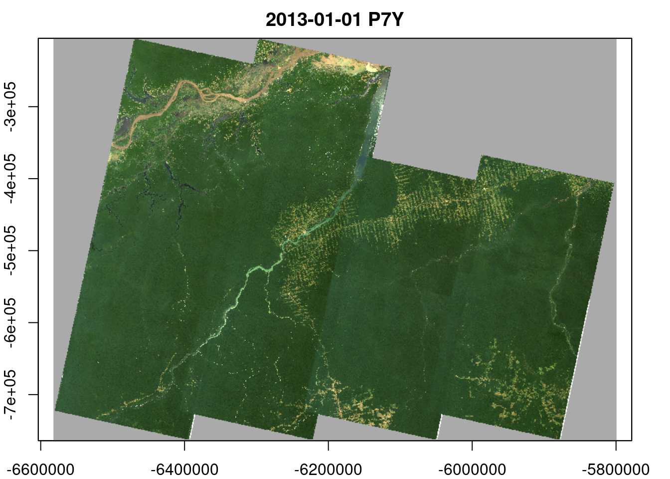
v= cube_view(extent=L8.col, dt="P1Y", dx=1000, dy=1000, 
             srs="EPSG:3857", aggregation = "median")
x = raster_cube(L8.col, v) 
x

A data cube proxy object

Dimensions:
                low              high count pixel_size chunk_size
t        2013-01-01        2019-12-31     7        P1Y          1
y -764014.387686915 -205014.387686915   559       1000        512
x -6582280.06164712 -5799280.06164712   783       1000        512

Bands:
        name offset scale nodata unit
1    AEROSOL      0     1    NaN     
2        B01      0     1    NaN     
3        B02      0     1    NaN     
4        B03      0     1    NaN     
5        B04      0     1    NaN     
6        B05      0     1    NaN     
7        B06      0     1    NaN     
8        B07      0     1    NaN     
9   PIXEL_QA      0     1    NaN     
10 RADSAT_QA      0     1    NaN     

Step 5: Process the data cube and plot

gdalcubes_options(parallel = 4)
x |>
  select_bands(c("B02","B03","B04")) |>
  reduce_time(c("median(B02)","median(B03)","median(B04)")) |>
  plot(x, rgb=3:1, zlim=c(0,1200))